The protein folding problem refers to the challenge : Can we predict a protein's structure completely from its sequence?. While this is possible using X-ray crystallography and Nuclear Magnetic Resonance (NMR), these techniques face challenges such as:
- low success rates in getting high quality protein crystals (for ex: intrinsically disordered proteins fall in this category. More details on how to grow crystals here),
- limitations on the protein sizes that can be crystallized (for ex: while individual proteins in the Nuclear Pore Complex (NPC) can be crystallized and examined, the overall assembly remains elusive to study via experimental techniques),
- tedious process with low throughput rates.
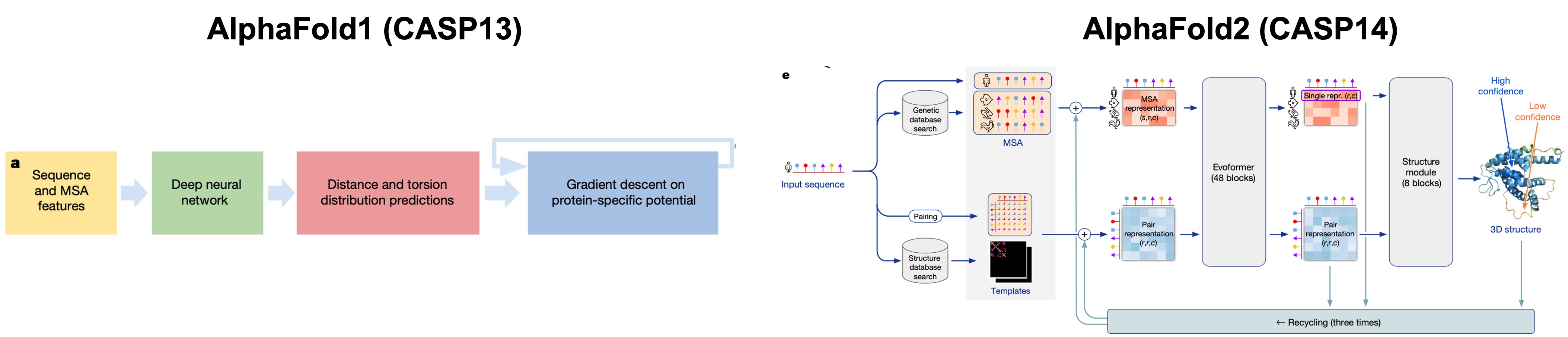
An alternative approach would be to simulate the protein folding process using computers. However, our current compute capabilities allow access to simulation times on the scale of 10s of nanoseconds, enabling folding simulations of only small proteins.[1] Google DeepMind's first iteration at this problem, called AlphaFold1, uses Convolutional Neural Networks (CNNs) to predict torsion and distance distributions (called distograms) from Multiple Sequence Alignment (MSA) features. Potentials were constructed based on these distributions and the initial structure from the predicted torsion and distance distributions was minimized using gradient descent.[2] Using this strategy the DeepMind team could predict accurate protein backbone structures.[2]
The following year the DeepMind team unveiled a more powerful model, based on the transformer architecture, that could now predict accurate protein side conformations as well. This model, called AlphaFold2, could predict structures with a median backbone accuracy of 0.96 Å r.m.s.d.95 (Cα root-mean-square deviation at 95% residue coverage) on the CASP14 test domains. In addition, most predicted structures had Template Modelling (TM) scores greater than 0.9.[3] AlphaFold2 marks the start of a series of computational models that predict protein structures on the scale of experimental accuracy.
AlphaFold3 (AF3) was released by the DeepMind team in 2023 and is their latest open source model as of date that goes beyond just predicting protein structures and includes RNA, DNA, docking of ligands and ions, bio-molecular complexes and multimers.[4] In this technical blog I will go over some of the details of the model architecture, results on benchmarks and some of the limitations of this model.
The journey from token to structure
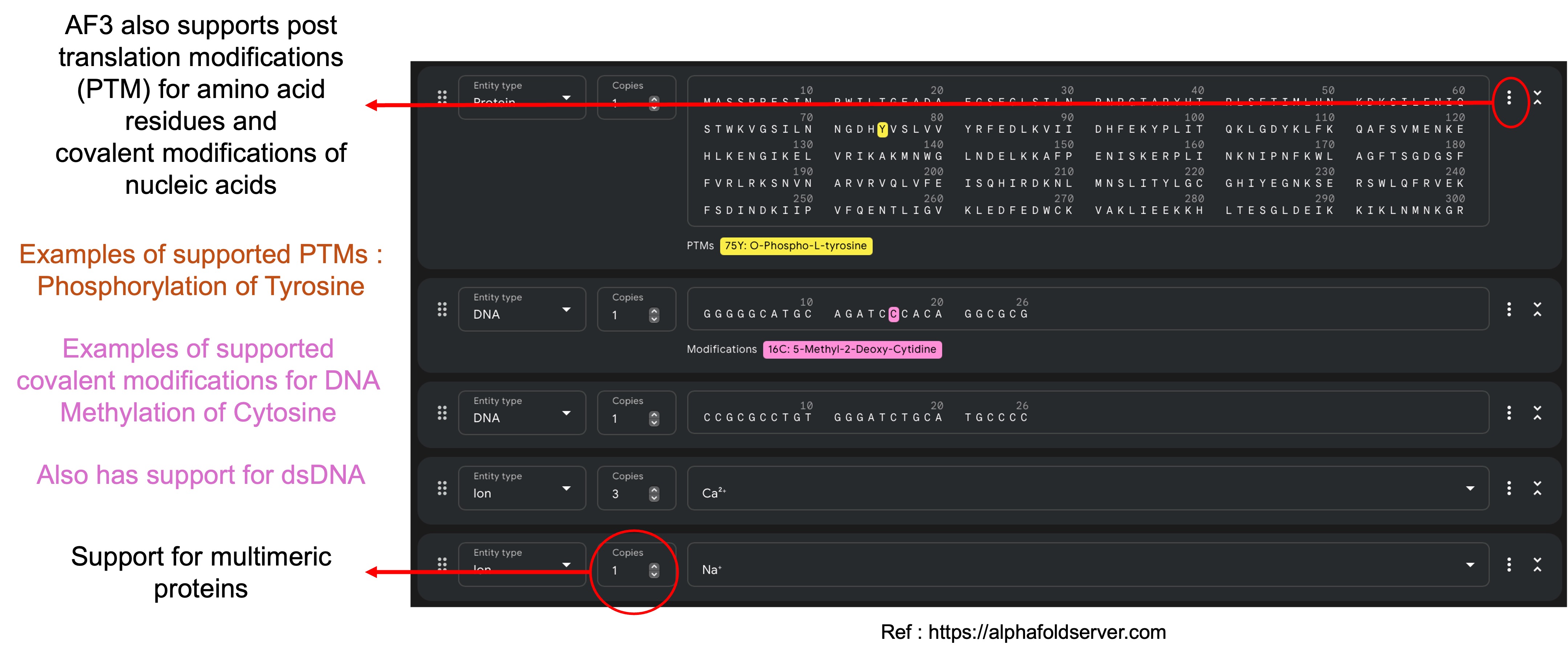
Below figure is a snapshot of the screen the user encounters when using the AlphaFold server. It provides a text box for the user to paste in their protein, DNA or RNA sequence and a dropdown menu to choose from the different types of ions and ligands AF3 supports.
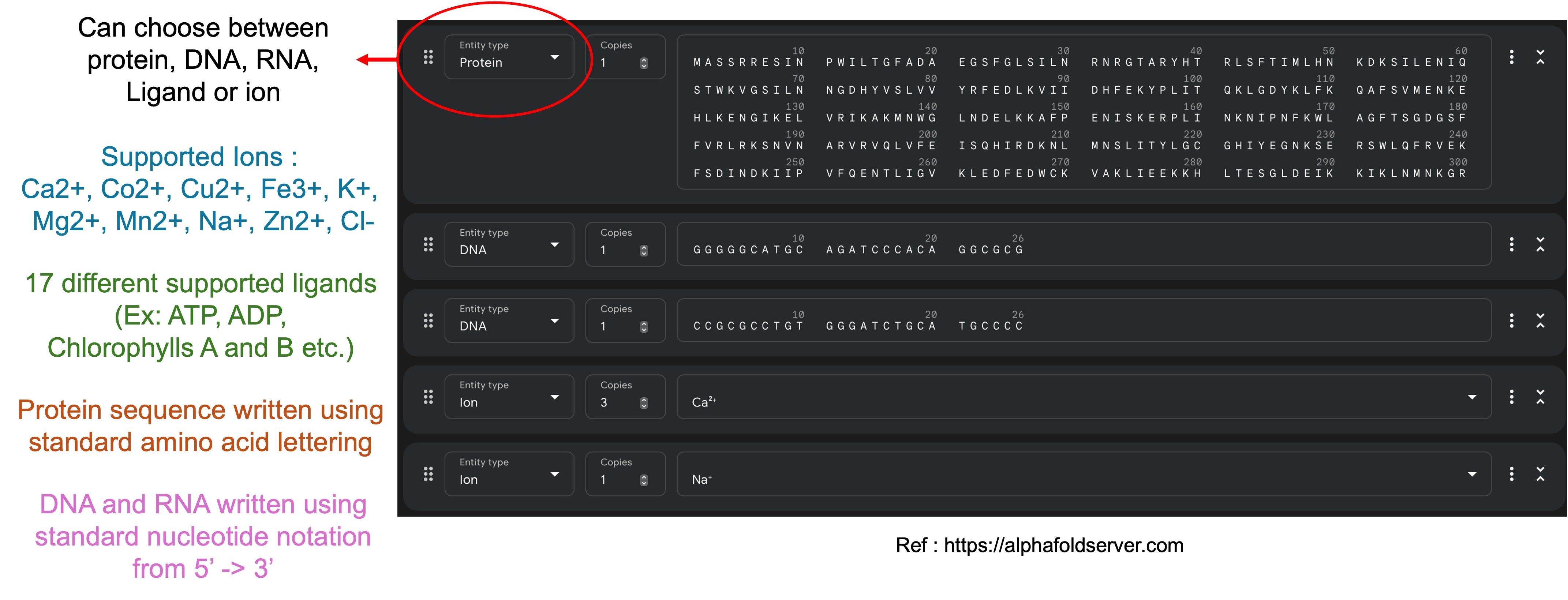
AF3 also provides supports for structure prediction of multimeric chains and for different post translation modifications of amino acid residues and DNA/RNA nucleotides.
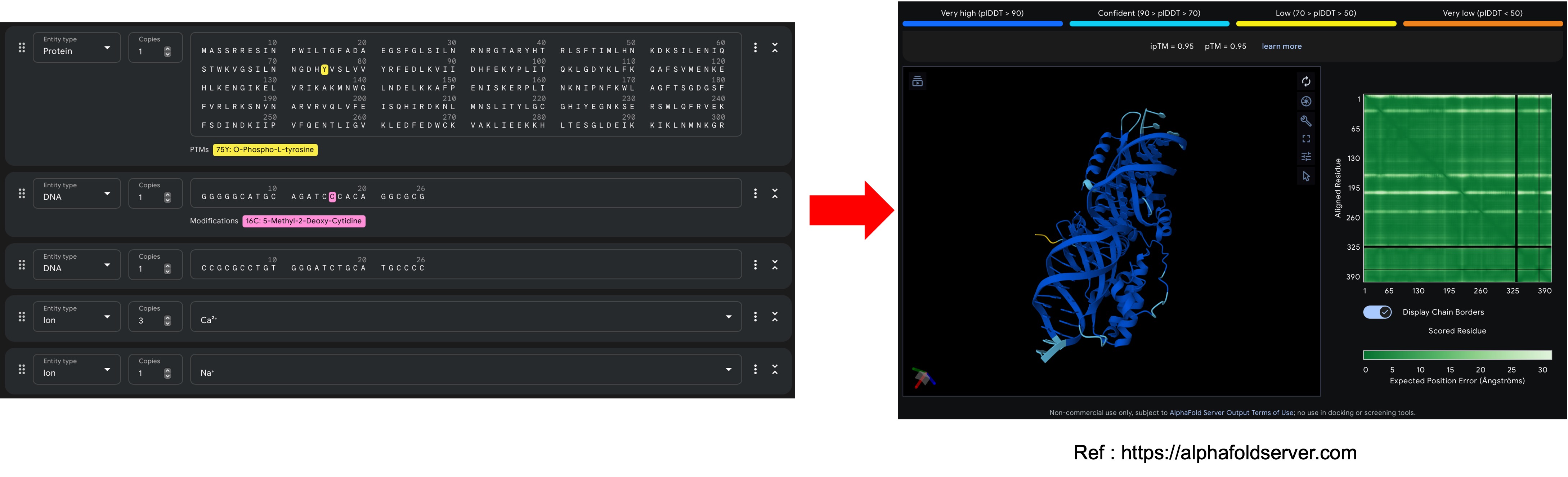
Once the user submits the job. AF3 runs the user input data through a data processing pipeline, generates features to feed the model and then predicts the 3D atomic coordinates and per atom confidence (pLDDT) and alignment metrics.
When the user submits the job on the AlphaFold server, AF3 runs a data processing pipeline where :
- input sequences are tokenized and features extracted from the tokenized sequences (Section 1.1),
- reference conformers generated for each residue/nucleotide (Section 1.2),
- MSA run on the input sequence and the search results are featurized (Section 1.3),
- template searches for single entities based on the retrieved MSA results (Section 1.4).
1.1. Tokenization of input sequences
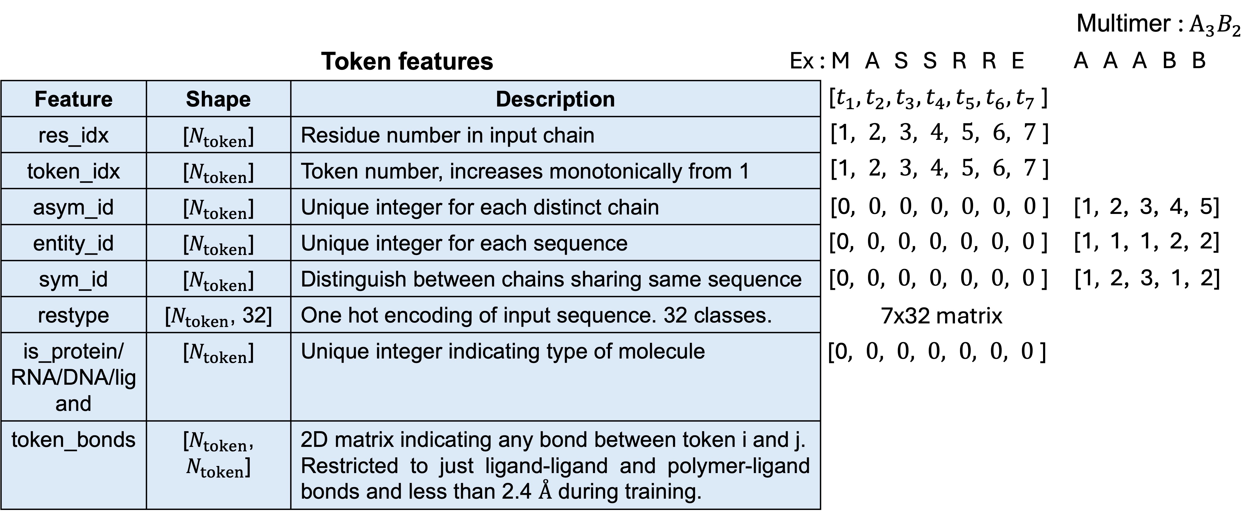
The amino acids, nucleotides, ligands and ions are represented using numerical representation called tokens. Each standard amino acid and nucleotide are represented using single tokens while modified amino acids, ligands and ions are tokenized per-atom. For example, Serine which is a standard amino acid is represented by 1 token while ibuprofen which contains 15 heavy atoms is represented using 15 tokens. There are in total 32 classes of molecules : 20 standard amino acids + 1 unknown, 4 standard DNA nucleotides + 1 unknown, 4 standard RNA nucleotides + 1 unknown, gap (from the MSA), ligands and ions are treated as unknown. Two examples are shown below, where in one case a protein chain is comprised of standard amino acids and another case consisting of multiple chains. The token features overall attempt to distinguish between the different amino acids and nucleotides in a chain from those present in different chains, as in the case of multimers. The token_bonds feature is a 2D matrix which indicates whether a bond exists between token i and j and is restricted to just inter ligand bonds and bonds between ligand and polymer which are less than 2.4 Å.
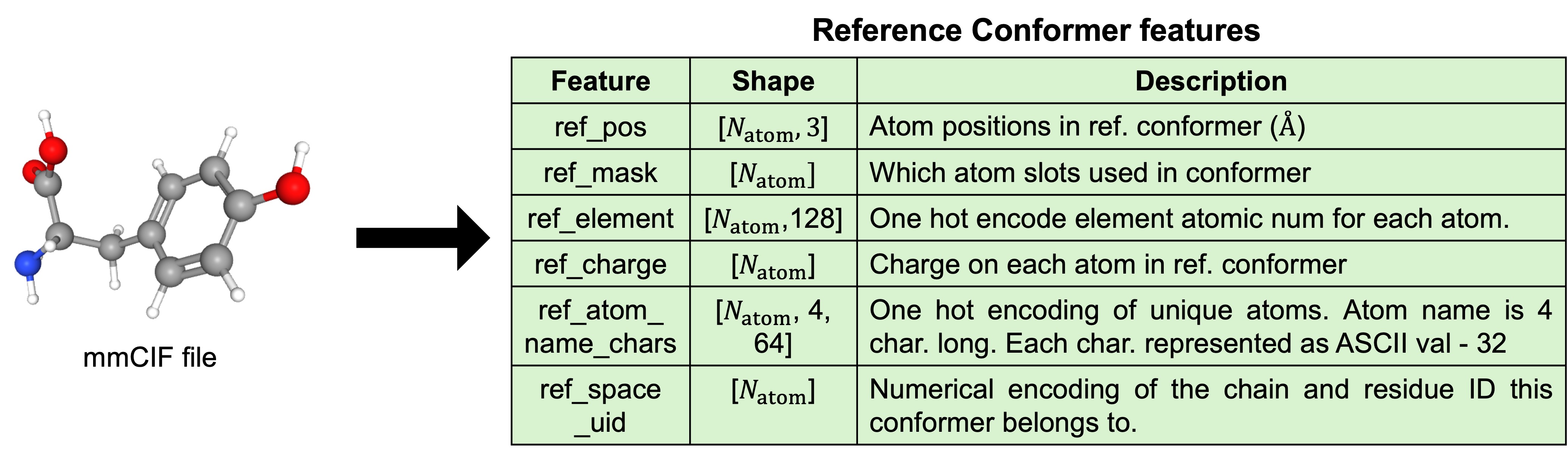
1.2. Generation of reference conformers (Training only)
Reference conformers for each monomer in the chains are created using RDKit's ETKDG3 confomer generation algorithm. Data from the mmCIF file is used to create a set of features shown in Figure 6. Conformer generation done only during training. At inference time, a dummy CIF with all atom coordinates zeroed is used.
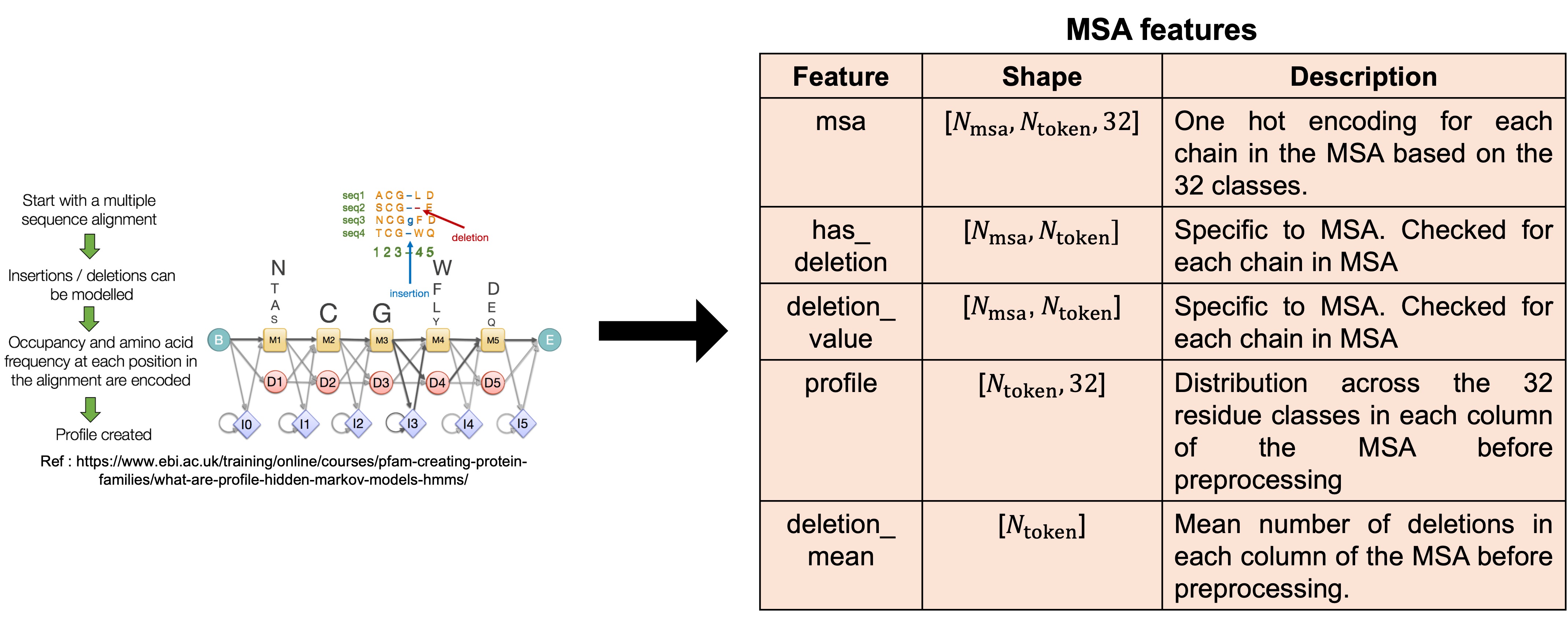
1.3. Multiple Sequence Alignment (MSA) searches
The process of aligning 2 or more protein, DNA or RNA sequences to maximize regions of sequence similarity is called Multiple Sequence Alignment (MSA). More details on MSA can be found in this blogpost. MSA is useful in structure prediction as correlated mutations are evolutionary signals that AF3 can use to infer whether a pair of residues are in close proximity with each other. AF3 uses Hidden Markov Models (HMMs) to build the MSA for the query sequence because traditional sequence alignment algorithms do not provide site specific substitution probabilities. Unlike traditional HMMs which take the form of cyclic graphs, HMMs from MSA, also called profiles, have a directional information flow from left to right. An example HMM is shown in Figure 7 where starting from the left end of the sequence, the arrows indicate the most probable state to enter next. The states are indicated as M, D and I which represent an amino acid, deletion or insertion state respectively.
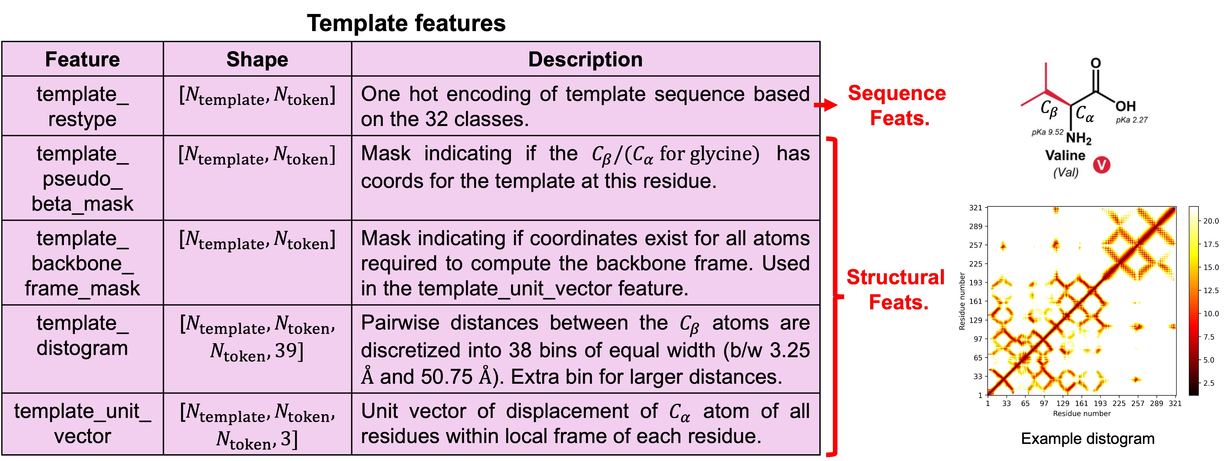
1.4. Creating structural priors by searching for templates
Using the constructed MSA profile in the previous step, AF3 next runs a search across genetic databases to find structural priors for the input sequence. This is done only for individual chains so the model does not know how different chains are in proximity with each other. AF3 uses upto 4 templates during training and inference. The template features can be divided based on sequence and structure. While AF1 predicts distograms, AF3 uses distograms for the template as an input.
2. High Level Overview of AF3 Architecture
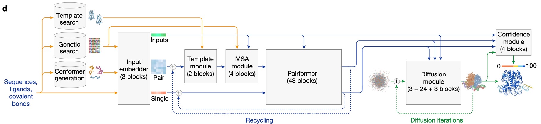
Okay so far we have collected the data and featurized it. Now we are ready to pass this data through the AF3 model and predict 3D structures and confidence metrics. The below model diagram shows the flow of information between the different AF3 model components. In the following sections I will give a high level overview about the functions of the Pairformer and Diffusion module. These modules refine two intermediate representations called the pair and single representations which are constructed by the Input Embedder module.
2.1. The Pair and Single Representations
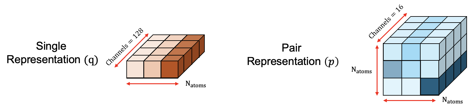
The pair and single representations operate on a fine-grained and coarse-grained scale. On the fine-grained scale the single representation ql is initialized by encoding the atomic positions and properties for each atom through a linear transformation into a 2D embedding. The number of channels controls the amount of information that can be stored in each atom's embedding as shown in Figure 10. The fine-grained pair representation plm is initialized by first encoding the inverse squared distances between atoms l and m, then the atom l and atom m features, and finally refined by passing through a Multi Layer Perceptron (MLP). Pair wise atom relationships are encoded within the 16 channels of plm as shown in Figure 10. Pair wise atom information is also added to ql by passing through Masked Attention and Conditioned Transition blocks 3 times.
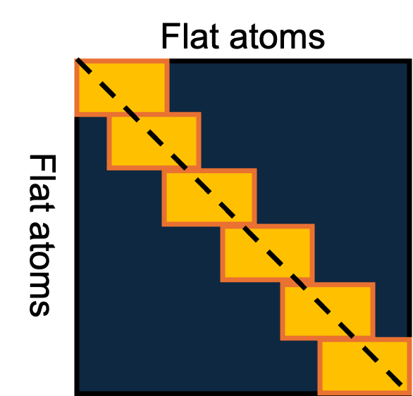
Masked Attention is performed by representing the whole structure as a flat list of atoms then for each subset of 32 atoms in the structure, the model focuses on the nearby 128 atoms. This restriction, while sub-optimal, was done to ensure that the memory and compute costs are kept within practical limits. The masked attention operation is performed by first computing the full affinity matrix $q_i^Tk_j$ and then adding the neighborhood mask $\beta_{ij}$ to realize the attentions only in yellow rectangular boxes as shown in Figure 11.
Attention $A_{ij}^h$ between atom $i$ and atom $j$, in attention head $h$, using neighborhood mask $\beta_{ij}$ is computed as
\[A_{ij}^h = \textrm{softmax} ( \frac{1}{\sqrt{c}} q_{i}^{h^T} k_{j}^h + \textrm{LinearNoBias}(z_{ij}) + \beta_{ij} ) v_{j}^h\]The query $q$, key $k$ and value $v$ arrays are computed from atom-level single representations $q_{i}$ and $q_{j}$, respectively. $c$ is computed as the dimensionality/number of channels in $q_{i}$ (i.e 128) divided by the number of attention heads (4). The attention is then gated and then linearly projected into the appropriate dimensionality and then passed onto the Conditioned Transition block.
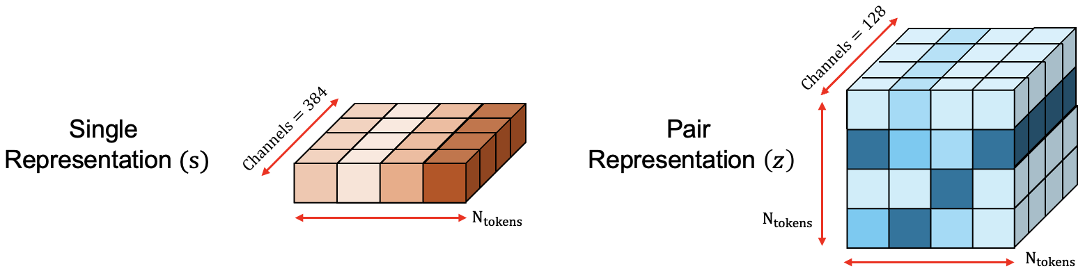
On the coarse grained scale the single $s_i$ and pair $z_{ij}$ representations encode residue level and inter-residue relationships, respectively. This enables the model to reason on a global/structural level. $s_i$ is initialized by averaging over all atom-level representations $q_l$ in the residue and then concatenated with the residue_type, profile and deletion_mean features. This creates the intermediate $s_{i}^{\rm{inputs}}$ representation which is then subsequently linearly projected into 384 channels to create $s_{i}$ as shown in Figure 12. $z_{ij}$ is initialized from the single representations $s_{i}$ and $s_{j}$ by linearly projecting into 128 channels, followed by refinement through the **Relative Positional Encoding** block, which helps differentiate between residues belonging to different chains. Finally, chemically connectivity information between tokens is added.
$s_i$ and $z_{ij}$ are continuously updated as they are passed through multiple module layers until they reach the Diffusion Module where starting from gaussian distributed 3D atomic coordinates, the module iteratively denoises to predict atomic coordinates conditioned based on the refined $s_i$ and $z_{ij}$.
2.2. The Pairformer module
The Pairformer module is the second last module in the AF3 model architecture which is responsible for constraining the values of the pair embeddings based on directional geometric reasoning. The triangle multiplicative and self attention updates are based on the triangle inequality. The transition block linearly transforms the output from the triangular update blocks into 4x larger dimensional space, applies a non-linear transformation through the swish activation function and then performs a linear dimensionality reduction back to 128 channels.
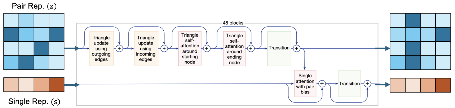
To understand how the triangle updates work its best to view the matrix representation as a directed graph. Directed edges are required since the pair representations $z_{ij}$ and $z_{ji}$ are not commutative. Figure 14 shows an example of how to construct the directed graph using tokens $i$, $j$ and $k$ as the graph nodes. The pair representation $z_{ij}$ is represented as a directed edge drawn from node $i$ to node $j$. To form the triangle, directed edges can be drawn starting from nodes $i$ and $j$ and ending at node $k$. These are called as outgoing edges. Node $k$ is varied according to the tokens in the input sequence. In the pair representation, this can be understood as varying $k$ while keeping the row indices $i$ and $j$ fixed. The other way to draw the directed graph is to start from node $k$ and draw directed edges towards node $i$ and node $j$, as depicted in bottom of Figure 14. These are called as incoming edges. Again while fixing node $i$ and node $j$, we can vary node $k$. In the pair representation, this can be understood as varying $k$ while keeping the column indices $i$ and $j$ fixed.
For each of the triangles formed with the directed edges we can apply the triangle inequality. For example for node $k_{1}$, the triangle inequality is $d_{ij} < d_{ik_1} + d_{jk_1}$. We can sum individual triangle updates which gives the final equation shown to the left in Figure 14. However, the actual implementation details are difficult to understand and not properly documented. I believe to improve the speed of triangular updates, AF3 uses Hadamard products instead of computing sums. AF3 also uses sigmoid gates to control the flow of information and lets the model identify which updates are more important. However, details such as why the use of two vectors $a$ and $b$ is not clear. The complete algorithm for computing triangular multiplicative updates for the outgoing edges is as follows :
def TriangleMultiplicationOutgoing({zij}, c=128):
    # This operation outputs two new vectors aik and bik
    # to use in the Hadamard product using 2 linear NNs.
    # aik, bik ∈ ℝ^128
    aik, bik = sigmoid(LinearNoBias(zik)) ⨀ LinearNoBias(zik)
    # Compute ajk and bjk (ajk, bjk ∈ ℝ^128)
    ajk, bjk = sigmoid(LinearNoBias(zjk)) ⨀ LinearNoBias(zjk)

    # Sigmoid gating of the output from the Hadamard Product.
    gij = sigmoid(LinearNoBias(LayerNorm(zij)))

    # Compute update
    𝑧ij_update = gij ⨀ LinearNoBias(LayerNorm(sum_k(aik ⨀ bjk)))
The triangular multiplicative updates using the incoming edges follows a similar algorithm with the computation of $a_{ik}$ and $b_{jk}$ replaced with computation of $a_{ki}$ and $b_{kj}$.
In the triangle self attention block AF3 first computes attention between each $z_{ij}$ and $z_{ik}$ pair representation. To complete the triangle, AF3 computes an attention bias $b_{jk}$ using $z_{jk}$. These operations are called triangle self attention around the "starting node" since graphically it can be visualized as drawing directed edges starting from node $i$ to every other other token in the sequence (i.e node $k$) as depicted in Figure 15 (left). $z_{ij}$ is used to compute the query array $q_{ij}$ while $z_{ik}$ is used to compute the key $k_{ik}$ and value $v_{ik}$ arrays which together with the bias term $b_{jk}$ is used to compute self attention $$ a_{ijk}^h = \textrm{softmax}_{k} ( \frac{1}{\sqrt{c}} q_{ij}^{h^T} k_{ik}^h + b_{jk}^{h} ) v_{ik}^h . $$ AF3 uses multi-headed attention and the superscript $h$ is used to index the attention head. In multi-headed attention, each attention head is allowed to specialize attention on different components of the input sequence, in this case focus on different aspects of the information stored in the channels of the pair representations. The dot product between $q_{ij}^{h}$ and $k_{ik}^h$ is scaled down by the dimensionality $c$ of the query, key and value arrays which is set to 32. In the second self attention block, AF3 computes attention between the $z_{ij}$ and $z_{kj}$ pair representations. To complete the triangle, AF3 computes an attention bias $b_{ki}$ using $z_{ki}$. These operations are called triangle self attention around the "ending node" since graphically it can be visualized as drawing directed edges starting from different $k$ nodes and ending at the node $j$ as depicted in Figure 15 (right).
The pesudocodes for triangle self attention about the "starting" and "ending" nodes are similar so I only present one of them. The only difference is that the computation of $k_{ik}$, $v_{ik}$ and $b_{jk}$ in TriangleAttentionStartingNode is replaced with computation of $k_{ki}$, $v_{ki}$ and $b_{kj}$ in TriangleAttentionEndingNode.
def TriangleAttentionStartingNode({zij}, c=32, Nhead=4):
    # Normalize the inputs
    zij ← LayerNorm(zij)gem
    zik ← LayerNorm(zik)
    zjk ← LayerNorm(zjk)
    # Projecting zij into the query, key and value space using 3 linear NN.
    # qij_h, kij_h, vij_h ∈ ℝ^32 and h ∈ {1 ... Nhead}
    qij_h, kij_h, vij_h = LinearNoBias(zij)
    # Projecting zij into the query, key and value space using 3 linear NN.
    qik_h, kik_h, vik_h = LinearNoBias(zik)
    # Computing the attention bias bjk (bjk_h ∈ ℝ^32)
    bjk_h = LinearNoBias(zjk)
    # Sigmoid gating information flow (gij_h ∈ ℝ^32)
    gij_h = sigmoid(LinearNoBias(zij))

    # Computing attention for each k token (aijk_h ∈ ℝ^32)
    # matmul(transpose(qij_h), kik_h) creates a 32 x 32 attention matrix
    aijk_h = softmax_k(1/sqrt(c) * matmul(transpose(qij_h), kik_h) + bjk_h)
    # Multiply with gate
    oij_h = gij_h ⨀ sum_k(matmul(vik_h, aijk_h))

    # Concatenate the outputs from each head and then project back to ℝ^128
    zij_update = LinearNoBias(concat(oij_h))
2.3. The Diffusion module
In AF2 the structure module used invariant point attention algorithm. This is replaced with a standard non-equivariant point-cloud diffusion model in AF3.
During training, 48 diffusion modules are trained in parallel. This is efficient as the diffusion module is much cheaper to train compared to the trunk of AF3. The prediction of denoised coordinates follows a Langevin type dynamics (Check out sampling from $q(x_{t-1}|x_t, x_0)$ from my diffusion module blog) which takes as input the noisy coordinates and the learned gradient of the data density (also called score). To generate noisy coordinates $\overrightarrow x_{l}^{\rm{noisy}}$, the 48 ground truth structures are randomly rotated and translated, $\overrightarrow x_l$. We also have to add gaussian noise $\overrightarrow \xi_{l}$ to the permuted coordinates which is sampled as $$ \overrightarrow \xi_{l} = \lambda \sqrt{\hat t^2 - c_{\tau - 1}^2} . N(\overrightarrow 0, I_{3}) $$ with $\lambda$ being the noise scale set at 1.003 and $\hat t$ defined as $$ \hat t = c_{\tau - 1}(\gamma + 1). $$ $c_{\tau - 1}$ is the noise sampled from the schedule $$ c_{\tau} \sim \sigma_{\rm{data}}*\exp(-1.2 + 1.5*N(0, 1)) $$ during training and $\gamma$ controls amount of conditional noise that is added. If $c_{\tau}$ is greater than $\gamma_{\text{min}}$ then $\gamma$ is set to a predefined value of 0.8. If its less then it is set to 0. When the coordinate noise $\overrightarrow \xi_{l}$ is low, the diffusion module is trained to get the local stereochemistry correct while when $\overrightarrow \xi_{l}$ is high, more emphasis is put on getting the global structure correct. Thus without any torsion-based parametrizations and stereochemical losses, just by varying the noise levels, AF3 is able to learn these concepts internally. During training, a short/mini rollout is performed for 20 steps where the module's predictions are fed back as input to predict a new set of denoised atomic coordinates as depicted in Figure 16. During inference a longer rollout is performed for 200 steps with the noise schedule $[c_1, c_2 \dots c_{T}]$ defined as follows $$ c_{t} \sim \sigma_{\rm{data}}*(s_{\rm{max}}^{\frac{1}{p}} + t*(s_{\rm{min}}^{\frac{1}{p}} - s_{\rm{max}}^{\frac{1}{p}}))^{p}. $$ $\sigma_{\rm{data}}$ in both the training noise and inference noise schedule is set to 16, $p$ is set to 7, $s_{\rm{max}}$ and $s_{\rm{min}}$ are set to 160 and $4.10^{-4}$ respectively. $t$ is step size starting from 0 with increments of 1/200.
In the update equation multiplying $dt$ with the score computes the updates to the atomic coordinates. $\eta$ acts as a learning rate, controlling the magnitude of the coordinate update. In the AF3 paper it is set to 1.5.
How does the Diffusion Module work ?
3. Training Losses
4. Benchmarks
References
[1] Scheraga, H. A.; Khalili, M.; Liwo, A. Protein-Folding Dynamics: Overview of Molecular Simulation Techniques. Annu. Rev. Phys. Chem. 2007, 58 (1), 57–83.https://doi.org/10.1146/annurev.physchem.58.032806.104614.
[2] Senior, A. W.; Evans, R.; Jumper, J.; Kirkpatrick, J.; Sifre, L.; Green, T.; Qin, C.; Žídek, A.; Nelson, A. W. R.; Bridgland, A.; Penedones, H.; Petersen, S.; Simonyan, K.; Crossan, S.; Kohli, P.; Jones, D. T.; Silver, D.; Kavukcuoglu, K.; Hassabis, D. Improved Protein Structure Prediction Using Potentials from Deep Learning. Nature 2020, 577 (7792), 706–710.https://doi.org/10.1038/s41586-019-1923-7.
[3] Jumper, J.; Evans, R.; Pritzel, A.; Green, T.; Figurnov, M.; Ronneberger, O.; Tunyasuvunakool, K.; Bates, R.; Žídek, A.; Potapenko, A.; Bridgland, A.; Meyer, C.; Kohl, S. A. A.; Ballard, A. J.; Cowie, A.; Romera-Paredes, B.; Nikolov, S.; Jain, R.; Adler, J.; Back, T.; Petersen, S.; Reiman, D.; Clancy, E.; Zielinski, M.; Steinegger, M.; Pacholska, M.; Berghammer, T.; Bodenstein, S.; Silver, D.; Vinyals, O.; Senior, A. W.; Kavukcuoglu, K.; Kohli, P.; Hassabis, D. Highly Accurate Protein Structure Prediction with AlphaFold. Nature 2021, 596 (7873), 583–589. https://doi.org/10.1038/s41586-021-03819-2.
[4] Abramson, J.; Adler, J.; Dunger, J.; Evans, R.; Green, T.; Pritzel, A.; Ronneberger, O.; Willmore, L.; Ballard, A. J.; Bambrick, J.; Bodenstein, S. W.; Evans, D. A.; Hung, C.-C.; O’Neill, M.; Reiman, D.; Tunyasuvunakool, K.; Wu, Z.; Žemgulytė, A.; Arvaniti, E.; Beattie, C.; Bertolli, O.; Bridgland, A.; Cherepanov, A.; Congreve, M.; Cowen-Rivers, A. I.; Cowie, A.; Figurnov, M.; Fuchs, F. B.; Gladman, H.; Jain, R.; Khan, Y. A.; Low, C. M. R.; Perlin, K.; Potapenko, A.; Savy, P.; Singh, S.; Stecula, A.; Thillaisundaram, A.; Tong, C.; Yakneen, S.; Zhong, E. D.; Zielinski, M.; Žídek, A.; Bapst, V.; Kohli, P.; Jaderberg, M.; Hassabis, D.; Jumper, J. M. Accurate Structure Prediction of Biomolecular Interactions with AlphaFold 3. Nature 2024, 630 (8016), 493–500. https://doi.org/10.1038/s41586-024-07487-w.